| OpenCV Smoothing and Blurring | 您所在的位置:网站首页 › blurring out › OpenCV Smoothing and Blurring |
OpenCV Smoothing and Blurring
|
Click here to download the source code to this post
In this tutorial, you will learn about smoothing and blurring with OpenCV. 
We will cover the following blurring operations Simple blurring (cv2.blur)Weighted Gaussian blurring (cv2.GaussianBlur)Median filtering (cv2.medianBlur)Bilateral blurring (cv2.bilateralFilter)By the end of this tutorial, you’ll be able to confidently apply OpenCV’s blurring functions to your own images. A dataset of images with different textures and details is beneficial for understanding the effects of smoothing and blurring. It allows us to see how these techniques can reduce noise and detail in images. Roboflow has free tools for each stage of the computer vision pipeline that will streamline your workflows and supercharge your productivity. Sign up or Log in to your Roboflow account to access state of the art dataset libaries and revolutionize your computer vision pipeline. You can start by choosing your own datasets or using our PyimageSearch’s assorted library of useful datasets. Bring data in any of 40+ formats to Roboflow, train using any state-of-the-art model architectures, deploy across multiple platforms (API, NVIDIA, browser, iOS, etc), and connect to applications or 3rd party tools. To learn how to perform smoothing and blurring with OpenCV, just keep reading. I’m pretty sure we all know what blurring is. Visually, it’s what happens when your camera takes a picture out of focus. Sharper regions in the image lose their detail. The goal here is to use a low-pass filter to reduce the amount of noise and detail in an image. Practically, this means that each pixel in the image is mixed in with its surrounding pixel intensities. This “mixture” of pixels in a neighborhood becomes our blurred pixel. While this effect is usually unwanted in our photographs, it’s actually quite helpful when performing image processing tasks. In fact, smoothing and blurring is one of the most common preprocessing steps in computer vision and image processing. For example, we can see that blurring is applied when building a simple document scanner on the PyImageSearch blog. We also apply smoothing to aid us in finding our marker when measuring the distance from an object to our camera. In both these examples the smaller details in the image are smoothed out and we are left with more of the structural aspects of the image. As we’ll see through this series of tutorials, many image processing and computer vision functions, such as thresholding and edge detection, perform better if the image is first smoothed or blurred. Why is smoothing and blurring such an important preprocessing operation?Smoothing and blurring is one of the most important preprocessing steps in all of computer vision and image processing. By smoothing an image prior to applying techniques such as edge detection or thresholding we are able to reduce the amount of high-frequency content, such as noise and edges (i.e., the “detail” of an image). While this may sound counter-intuitive, by reducing the detail in an image we can more easily find objects that we are interested in. Furthermore, this allows us to focus on the larger structural objects in the image. In the rest of this lesson we’ll be discussing the four main smoothing and blurring options that you’ll often use in your own projects: Simple average blurringGaussian blurringMedian filteringBilateral filteringLet’s get started. Configuring your development environmentTo follow this guide, you need to have the OpenCV library installed on your system. Luckily, OpenCV is pip-installable: $ pip install opencv-contrib-pythonIf you need help configuring your development environment for OpenCV, I highly recommend that you read my pip install OpenCV guide — it will have you up and running in a matter of minutes. Having problems configuring your development environment? Figure 1: Having trouble configuring your dev environment? Want access to pre-configured Jupyter Notebooks running on Google Colab? Be sure to join PyImageSearch University — you’ll be up and running with this tutorial in a matter of minutes. Figure 1: Having trouble configuring your dev environment? Want access to pre-configured Jupyter Notebooks running on Google Colab? Be sure to join PyImageSearch University — you’ll be up and running with this tutorial in a matter of minutes.
All that said, are you: Short on time?Learning on your employer’s administratively locked system?Wanting to skip the hassle of fighting with the command line, package managers, and virtual environments?Ready to run the code right now on your Windows, macOS, or Linux systems?Then join PyImageSearch University today! Gain access to Jupyter Notebooks for this tutorial and other PyImageSearch guides that are pre-configured to run on Google Colab’s ecosystem right in your web browser! No installation required. And best of all, these Jupyter Notebooks will run on Windows, macOS, and Linux! Project structureBefore we can learn how to apply blurring with OpenCV, let’s first review our project directory structure. Start by accessing the “Downloads” section of this tutorial to retrieve the source code and example image: $ tree . --dirsfirst . ├── adrian.png ├── bilateral.py └── blurring.py 0 directories, 3 filesOur first script, blurring.py, will show you how to apply an average blur, Gaussian blur, and median blur to an image (adrian.png) using OpenCV. The second Python script, bilateral.py, will demonstrate how to use OpenCV to apply a bilateral blur to our input image. Average blurring ( cv2.blur )The first blurring method we are going to explore is averaging. An average filter does exactly what you think it might do — takes an area of pixels surrounding a central pixel, averages all these pixels together, and replaces the central pixel with the average. By taking the average of the region surrounding a pixel, we are smoothing it and replacing it with the value of its local neighborhood. This allows us to reduce noise and the level of detail, simply by relying on the average. Remember when we discussed kernels and convolutions? Well, it turns out that we can use kernels for not only edge detection and gradients, but for averaging as well! To accomplish our average blur, we’ll actually be convolving our image with an  and and  are both odd integers. are both odd integers.
This kernel is going to slide from left-to-right and from top-to-bottom for each and every pixel in our input image. The pixel at the center of the kernel (and hence why we have to use an odd number, otherwise there would not be a true “center”) is then set to be the average of all other pixels surrounding it. Let’s go ahead and define a
Notice how each entry of the kernel matrix is uniformly weighted — we are giving equal weight to all pixels in the kernel. An alternative is to give pixels different weights, where pixels farther from the central pixel contribute less to the average; we’ll discuss this method of smoothing in the Gaussian blurring section of this lesson. We could also define a
This kernel takes more pixels into account for the average, and will blur the image more than a Hence, this brings us to an important rule: as the size of the kernel increases, so will the amount in which the image is blurred. Simply put: the larger your smoothing kernel is, the more blurred your image will look. To investigate this notion, let’s explore some code. Open the blurring.py file in your project directory structure and let’s get to work: # import the necessary packages import argparse import cv2 # construct the argument parser and parse the arguments ap = argparse.ArgumentParser() ap.add_argument("-i", "--image", type=str, default="adrian.png", help="path to input image") args = vars(ap.parse_args())Lines 2 and 3 import our required packages while Lines 6-9 parse our command line arguments. We only need a single argument, --image, which is the path to our input image on disk that we wish to apply smoothing and blurring to. By default, we set this argument to adrian.png. Let’s now load our input image from disk: # load the image, display it to our screen, and initialize a list of # kernel sizes (so we can evaluate the relationship between kernel # size and amount of blurring) image = cv2.imread(args["image"]) cv2.imshow("Original", image) kernelSizes = [(3, 3), (9, 9), (15, 15)] # loop over the kernel sizes for (kX, kY) in kernelSizes: # apply an "average" blur to the image using the current kernel # size blurred = cv2.blur(image, (kX, kY)) cv2.imshow("Average ({}, {})".format(kX, kY), blurred) cv2.waitKey(0)Lines 14 and 15 load our input image from disk and display it to our screen. We then define a list of kernelSizes on Line 16 — the sizes of these kernels increase progressively so we’ll be able to visualize the impact the kernel size has on the output image. From there, we start looping over each of the kernel sizes on Line 19. To average blur an image, we use the cv2.blur function. This function requires two arguments: the image we want to blur and the size of the kernel. As Lines 22-24 show, we blur our image with increasing sizes kernels. The larger our kernel becomes, the more blurred our image will appear. When you run this script you will receive the following output after applying the cv2.blur function: 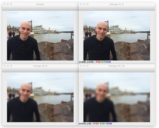 Figure 2: Smoothing an image using an average blur. Notice as how the kernel size increases, the image becomes progressively more blurred. Figure 2: Smoothing an image using an average blur. Notice as how the kernel size increases, the image becomes progressively more blurred.
On the top-left, we have our original input image. On the top-right, we have blurred it using a  and and  , the image becomes practically unrecognizable. , the image becomes practically unrecognizable.
Again, as the size of your kernel increases, your image will become progressively more blurred. This could easily lead to a point where you lose the edges of important structural objects in the image. Choosing the right amount of smoothing is critical when developing your own computer vision applications. While average smoothing was quite simple to understand, it also weights each pixel inside the kernel area equally — and by doing this it becomes easy to over-blur our image and miss out on important edges. We can remedy this problem by applying Gaussian blurring. Gaussian blurring ( cv2.GaussianBlur)Next up, we are going to review Gaussian blurring. Gaussian blurring is similar to average blurring, but instead of using a simple mean, we are now using a weighted mean, where neighborhood pixels that are closer to the central pixel contribute more “weight” to the average. And as the name suggests, Gaussian smoothing is used to remove noise that approximately follows a Gaussian distribution. The end result is that our image is less blurred, but more “naturally blurred,” than using the average method discussed in the previous section. Furthermore, based on this weighting we’ll be able to preserve more of the edges in our image as compared to average smoothing. Just like an average blurring, Gaussian smoothing also uses a kernel of and are odd integers.
However, since we are weighting pixels based on how far they are from the central pixel, we need an equation to construct our kernel. The equation for a Gaussian function in one direction is:
And it then becomes trivial to extend this equation to two directions, one for the x-axis and the other for the y-axis, respectively:
where  are the respective distances to the horizontal and vertical center of the kernel and are the respective distances to the horizontal and vertical center of the kernel and  is the standard deviation of the Gaussian kernel. is the standard deviation of the Gaussian kernel.
Again, as we’ll see in the code below, when the size of our kernel increases so will the amount of blurring that is applied to our output image. However, the blurring will appear to be more “natural” and will preserve edges in our image better than simple average smoothing: # close all windows to cleanup the screen cv2.destroyAllWindows() cv2.imshow("Original", image) # loop over the kernel sizes again for (kX, kY) in kernelSizes: # apply a "Gaussian" blur to the image blurred = cv2.GaussianBlur(image, (kX, kY), 0) cv2.imshow("Gaussian ({}, {})".format(kX, kY), blurred) cv2.waitKey(0)Lines 27 and 28 simply close all open windows and display our original image as a reference point. The actual Gaussian blur takes place on Lines 31-35 by using the cv2.GaussianBlur function. The first argument to the function is the image we want to blur. Then, similar to cv2.blur, we provide a tuple representing our kernel size. Again, we start with a small kernel size of The last parameter is our based on our kernel size.
In most cases, you’ll want to let your for yourself, I would suggest reading through the OpenCV documentation on cv2.GaussianBlur to ensure you understand the implications.
We can see the output of our Gaussian blur in Figure 3:  Figure 3: Applying Gaussian blurring. Figure 3: Applying Gaussian blurring.
Our images have less of a blur effect than when using the averaging method in Figure 2; however, the blur itself is more natural due to the computation of the weighted mean, rather than allowing all pixels in the kernel neighborhood to have equal weight. In general, I tend to recommend starting with a simple Gaussian blur and tuning your parameters as needed. While the Gaussian blur is slightly slower than a simple average blur (and only by a tiny fraction), a Gaussian blur tends to give much nicer results, especially when applied to natural images. Median blurring ( cv2.medianBlur )Traditionally, the median blur method has been most effective when removing salt-and-pepper noise. This type of noise is exactly what it sounds like: imagine taking a photograph, putting it on your dining room table, and sprinkling salt and pepper on top of it. Using the median blur method, you could remove the salt and pepper from your image. When applying a median blur, we first define our kernel size. Then, as in the averaging blurring method, we consider all pixels in the neighborhood of size  is an odd integer. is an odd integer.
Notice how, unlike average blurring and Gaussian blurring where the kernel size could be rectangular, the kernel size for the median must be square. Furthermore (unlike the averaging method), instead of replacing the central pixel with the average of the neighborhood, we instead replace the central pixel with the median of the neighborhood. The reason median blurring is more effective at removing salt-and-pepper style noise from an image is that each central pixel is always replaced with a pixel intensity that exists in the image. And since the median is robust to outliers, the salt-and-pepper noise will be less influential to the median than another statistical method, such as the average. Again, methods such as averaging and Gaussian compute means or weighted means for the neighborhood — this average pixel intensity may or may not be present in the neighborhood. But by definition, the median pixel must exist in our neighborhood. By replacing our central pixel with a median rather than an average, we can substantially reduce noise. Let’s now apply our median blur: # close all windows to cleanup the screen cv2.destroyAllWindows() cv2.imshow("Original", image) # loop over the kernel sizes a final time for k in (3, 9, 15): # apply a "median" blur to the image blurred = cv2.medianBlur(image, k) cv2.imshow("Median {}".format(k), blurred) cv2.waitKey(0)Applying a median blur is accomplished by making a call to the cv2.medianBlur function. This method takes two parameters: the image we want to blur and the size of our kernel. On Line 42 we start looping over (square) kernel sizes. We start off with a kernel size of 3 and then increase it to 9 and 15. The resulting median blurred images are then stacked and displayed to us can be seen in Figure 4:  Figure 4: Applying a median blur with progressively larger kernel sizes. Figure 4: Applying a median blur with progressively larger kernel sizes.
Notice that we are no longer creating a “motion blur” effect like in averaging and Gaussian blurring — instead, we are removing substantially more detail and noise. For example, take a look at the color of the rocks to the right of myself in the image. As our kernel size increases, detail and color on the rocks become substantially less pronounced. By the time we are using a The same can be said for my face in the image — as the kernel size increases, my face rapidly loses detail and practically blends together. The median blur is by no means a “natural blur” like Gaussian smoothing. However, for damaged images or photos captured under highly suboptimal conditions, a median blur can really help as a pre-processing step prior to passing the image along to other methods, such as thresholding and edge detection. Bilateral blurring ( cv2.bilateralFilter )The last method we are going to explore is bilateral blurring. Thus far, the intention of our blurring methods have been to reduce noise and detail in an image; however, as a side effect we have tended to lose edges in the image. To reduce noise while still maintaining edges, we can use bilateral blurring. Bilateral blurring accomplishes this by introducing two Gaussian distributions. The first Gaussian function only considers spatial neighbors. That is, pixels that appear close together in the Intuitively, this makes sense. If pixels in the same (small) neighborhood have a similar pixel value, then they likely represent the same object. But if two pixels in the same neighborhood have contrasting values, then we could be examining the edge or boundary of an object — and we would like to preserve this edge. Overall, this method is able to preserve edges of an image, while still reducing noise. The largest downside to this method is that it is considerably slower than its averaging, Gaussian, and median blurring counterparts. Let’s dive into the code for bilateral blurring. Open the bilateral.py file in your project directory structure and we’ll get to work: # import the necessary packages import argparse import cv2 # construct the argument parser and parse the arguments ap = argparse.ArgumentParser() ap.add_argument("-i", "--image", type=str, default="adrian.png", help="path to input image") args = vars(ap.parse_args())Lines 2 and 3 import our required Python packages while Lines 6-9 parse our command line arguments. Again, only a single argument is needed, --image, which is the path to the input image we wish to apply bilateral blurring to. Let’s now load our image from disk: # load the image, display it to our screen, and construct a list of # bilateral filtering parameters that we are going to explore image = cv2.imread(args["image"]) cv2.imshow("Original", image) params = [(11, 21, 7), (11, 41, 21), (11, 61, 39)] # loop over the diameter, sigma color, and sigma space for (diameter, sigmaColor, sigmaSpace) in params: # apply bilateral filtering to the image using the current set of # parameters blurred = cv2.bilateralFilter(image, diameter, sigmaColor, sigmaSpace) # show the output image and associated parameters title = "Blurred d={}, sc={}, ss={}".format( diameter, sigmaColor, sigmaSpace) cv2.imshow(title, blurred) cv2.waitKey(0)We then define a list of blurring parameters on Line 15. These parameters correspond to the diameter,  of the bilateral filter, respectively. of the bilateral filter, respectively.
From there, we loop over each of these parameter sets on Line 18 and apply bilateral filtering by making a call to the cv2.bilateralFilter on Line 21. Finally, Lines 24-27 display our blurred image to our screen. Let’s take a second and review the parameters we supply to cv2.bilateralFilter. The first parameter we supply is the image we want to blur. Then, we need to define the diameter of our pixel neighborhood — the larger this diameter is, the more pixels will be included in the blurring computation. Think of this parameter as a square kernel size. The third argument is our color standard deviation, denoted as  means that more colors in the neighborhood will be considered when computing the blur. If we let get too large in respect to the diameter, then we essentially have broken the assumption of bilateral filtering — that only pixels of similar color should contribute significantly to the blur. means that more colors in the neighborhood will be considered when computing the blur. If we let get too large in respect to the diameter, then we essentially have broken the assumption of bilateral filtering — that only pixels of similar color should contribute significantly to the blur.
Finally, we need to supply the space standard deviation, which we call means that pixels farther out from the central pixel diameter will influence the blurring calculation.
When you execute this script you’ll see the following output from bilateral filtering:  Figure 5: Applying bilateral filtering to our image. Figure 5: Applying bilateral filtering to our image.
On the top-left, we have our original input image. And on the top-right, we start with a diameter of  , and , and  . .
The effects of our blurring are not fully apparent yet, but if you zoom in on the rocks and compare them to our original image, you’ll notice that much of the texture has disappeared! The rocks appear much smoother, as if they have been eroded and smoothed over years and years of rushing water. However, the edges and boundaries between the lake and the rocks are clearly maintained. Now, take a look at the bottom-left where we have increased both jointly. At this point we can really see the effects of bilateral filtering.
The buttons on my black hoodie have practically disappeared and nearly all detail and wrinkles on my skin have been removed. Yet at the same time there is still a clear boundary between myself and the background of the image. If we were using an average or Gaussian blur, the background would be melding with the foreground. Finally, we have the bottom-right, where I have increased yet again, just to demonstrate how powerful of a technique bilateral filtering is.
Now nearly all detail and texture from the rocks, water, sky, and my skin and hoodie are gone. It’s also starting to look as if the number of colors in the image have been reduced. Again, this is an exaggerated example and you likely wouldn’t be applying this much blurring to an image, but it does demonstrate the effect bilateral filtering will have on your edges: dramatically smoothed detail and texture, while still preserving boundaries and edges. So there you have it — an overview of blurring techniques! If it’s not entirely clear when you will use each blurring or smoothing method just yet, that’s okay. We will be building on these blurring techniques substantially in this series of tutorials and you’ll see plenty of examples on when to apply each type of blurring. For the time being, just try to digest the material and store blurring and smoothing as yet another tool in your toolkit. OpenCV blurring resultsReady to run our smoothing and blurring scripts? Be sure to access the “Downloads” section of this tutorial to retrieve the source code and example image. You can then apply basic smoothing and blurring by executing the blurring.py script: $ python blurring.pyTo see the output of bilateral blurring, run the following command: $ python bilateral.pyThe output of these scripts should match the images and figures I have provided above. What's next? We recommend PyImageSearch University. Course information: 83 total classes • 113+ hours of on-demand code walkthrough videos • Last updated: December 2023 ★★★★★ 4.84 (128 Ratings) • 16,000+ Students EnrolledI strongly believe that if you had the right teacher you could master computer vision and deep learning. Do you think learning computer vision and deep learning has to be time-consuming, overwhelming, and complicated? Or has to involve complex mathematics and equations? Or requires a degree in computer science? That’s not the case. All you need to master computer vision and deep learning is for someone to explain things to you in simple, intuitive terms. And that’s exactly what I do. My mission is to change education and how complex Artificial Intelligence topics are taught. If you're serious about learning computer vision, your next stop should be PyImageSearch University, the most comprehensive computer vision, deep learning, and OpenCV course online today. Here you’ll learn how to successfully and confidently apply computer vision to your work, research, and projects. Join me in computer vision mastery. Inside PyImageSearch University you'll find: ✓ 83 courses on essential computer vision, deep learning, and OpenCV topics ✓ 83 Certificates of Completion ✓ 113+ hours of on-demand video ✓ Brand new courses released regularly, ensuring you can keep up with state-of-the-art techniques ✓ Pre-configured Jupyter Notebooks in Google Colab ✓ Run all code examples in your web browser — works on Windows, macOS, and Linux (no dev environment configuration required!) ✓ Access to centralized code repos for all 532+ tutorials on PyImageSearch ✓ Easy one-click downloads for code, datasets, pre-trained models, etc. ✓ Access on mobile, laptop, desktop, etc.Click here to join PyImageSearch University SummaryIn this tutorial, we learned how to smooth and blur images using OpenCV. We started by discussing the role kernels play in smoothing and blurring. We then reviewed the four primary methods to smooth an image in OpenCV: Simple average blurringGaussian blurringMedian filteringBilateral filteringThe simple average method is fast, but may not preserve edges in images. Applying a Gaussian blur is better at preserving edges, but is slightly slower than the average method. A median filter is primarily used to reduce salt-and-pepper style noise as the median statistic is much more robust and less sensitive to outliers than other statistical methods such as the mean. Finally, the bilateral filter preserves edges, but is significantly slower than the other methods. Bilateral filtering also boasts the most parameters to tune which can become a nuisance to tune correctly. In general, I recommend starting with a simple Gaussian blur to obtain a baseline and then going from there. To download the source code to this post (and be notified when future tutorials are published here on PyImageSearch), simply enter your email address in the form below! What's next? We recommend PyImageSearch University. Course information: 83 total classes • 113+ hours of on-demand code walkthrough videos • Last updated: December 2023 ★★★★★ 4.84 (128 Ratings) • 16,000+ Students EnrolledI strongly believe that if you had the right teacher you could master computer vision and deep learning. Do you think learning computer vision and deep learning has to be time-consuming, overwhelming, and complicated? Or has to involve complex mathematics and equations? Or requires a degree in computer science? That’s not the case. All you need to master computer vision and deep learning is for someone to explain things to you in simple, intuitive terms. And that’s exactly what I do. My mission is to change education and how complex Artificial Intelligence topics are taught. If you're serious about learning computer vision, your next stop should be PyImageSearch University, the most comprehensive computer vision, deep learning, and OpenCV course online today. Here you’ll learn how to successfully and confidently apply computer vision to your work, research, and projects. Join me in computer vision mastery. Inside PyImageSearch University you'll find: ✓ 83 courses on essential computer vision, deep learning, and OpenCV topics ✓ 83 Certificates of Completion ✓ 113+ hours of on-demand video ✓ Brand new courses released regularly, ensuring you can keep up with state-of-the-art techniques ✓ Pre-configured Jupyter Notebooks in Google Colab ✓ Run all code examples in your web browser — works on Windows, macOS, and Linux (no dev environment configuration required!) ✓ Access to centralized code repos for all 532+ tutorials on PyImageSearch ✓ Easy one-click downloads for code, datasets, pre-trained models, etc. ✓ Access on mobile, laptop, desktop, etc.Click here to join PyImageSearch University  Download the Source Code and FREE 17-page Resource Guide
Enter your email address below to get a .zip of the code and a FREE 17-page Resource Guide on Computer Vision, OpenCV, and Deep Learning. Inside you'll find my hand-picked tutorials, books, courses, and libraries to help you master CV and DL! |


![K = \displaystyle\frac{1}{9} \left[\begin{tabular}{ccc}1 & 1 & 1\\ 1 & 1 & 1\\ 1 & 1 & 1\end{tabular}\right]](https://b2633864.smushcdn.com/2633864/wp-content/latex/23d/23d5e60dfcfeb2558c1905bf69785719-ffffff-000000-0.png?size=142x60&lossy=2&strip=1&webp=1 "K = \displaystyle\frac{1}{9} \left[\begin{tabular}{ccc}1 & 1 & 1\\ 1 & 1 & 1\\ 1 & 1 & 1\end{tabular}\right]")

![K = \displaystyle\frac{1}{25} \left[\begin{tabular}{ccccc}1 & 1 & 1 & 1 & 1\\ 1 & 1 & 1 & 1 & 1\\ 1 & 1 & 1 & 1 & 1\\ 1 & 1 & 1 & 1 & 1\\ 1 & 1 & 1 & 1 & 1\end{tabular}\right]](https://b2633864.smushcdn.com/2633864/wp-content/latex/712/7128697198112f30c8110260e1631a1d-ffffff-000000-0.png?size=200x100&lossy=2&strip=1&webp=1 "K = \displaystyle\frac{1}{25} \left[\begin{tabular}{ccccc}1 & 1 & 1 & 1 & 1\\ 1 & 1 & 1 & 1 & 1\\ 1 & 1 & 1 & 1 & 1\\ 1 & 1 & 1 & 1 & 1\\ 1 & 1 & 1 & 1 & 1\end{tabular}\right]")
 = \displaystyle\frac{1}{\displaystyle\sqrt{2\pi\sigma}}e^{-\frac{x^{2}}{2\sigma^{2}}}")
 = \displaystyle\frac{1}{2\pi\sigma}e^{-\frac{x^{2} + y^{2}}{2\sigma^{2}}}")


")

【本文地址】